Fitting seasonal data

For this demonstration we use length data for the sole, Solea solea, a flatfish. The data set was collected over a 25 year period in the Bristol Channel, England. Two data sets have been prepared as follows.

sole monthly.csv is a file giving the mean age of sole from an age of 0.16667 years (2 months) to 3,5 years of age. Note that age is expressed in fractions of a year, this is required when fitting a seasonal model using Growth II.

individual sole lengths.csv is a file holding the individual lengths and ages of sole.

Use File|Open to find and open sole monthly.csv (saved by default during installation in the folder C:\Program files\GrowthII\GrowthDemoData)

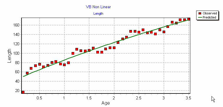
Once the data set has been opened, Growth II will immediately fit a von Bertalanffy growth curve to the data and plot the result:

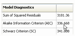
A brief glance at this graph and the Regression diagnostics in the grid below shows that the von Bertalanffy gives a fit that does pass through the scatter of points, but there is a clear periodic oscillation that the model fails to fit (note the size of the Akaike Information Criterion, AIC = 336.8). This number will be useful later to compare the models:

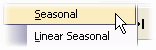
We will now get Growth II to fit a seasonally adjusted von Bertalanffy. From the Seasonal Age/Size drop-down select Seasonal

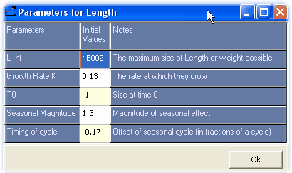
This will run a non-linear curve fitting routine to fit a seasonally adjusted von Bertalanffy model. Growth II immediately opens a dialogue box showing the initial guesses (shown below) for the 5 parameters needed for this model. The program needs initial guesses as it solves the non-linear regression using the Levenberg-Marquardt method. While the initial guesses can and sometimes have to be changed to get a solution, it is sensible to first try the defaults you are given.

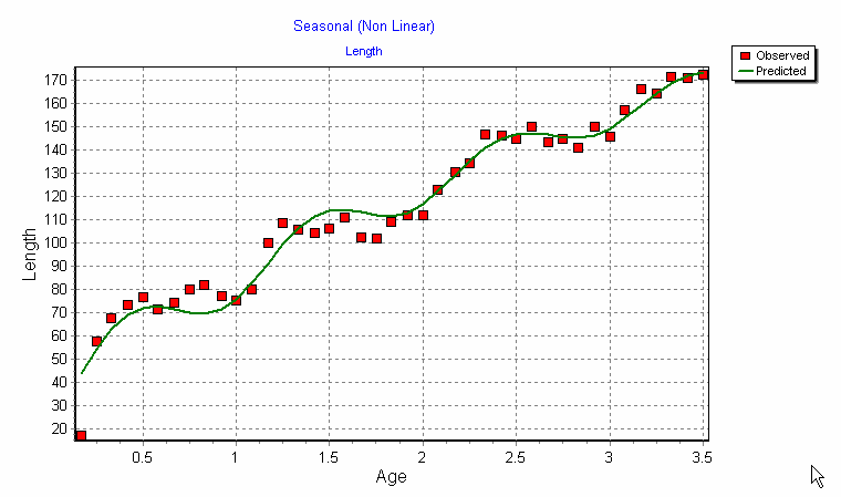
Click on OK and the fit is immediately presented. The plot shows the observed data and the fitted curve.

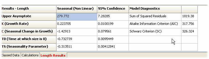
Below the plot are presented the the parameter estimates, their 95% confidence intervals.

The fitted model has an upper asymptote (called L infinity in fisheries science) of 279.77 cms with 95% confidence intervals of 279.77-7.28 = 272.49 cms and 279.77+7.28 = 287.05.

The growth rate K has units of Year-1.

C, the seasonal parameter has an absolute magnitude greater than 1, this indicates that the model predicts that the sole shrink during the winter. While individual fish do not shrink, close examination of the data does indicate that the average size does decline during the winter, this is probably because the larger fish migrate offshore and are not included in the winter samples.

The Akaike Information Criterion, AIC = 326.324 which is lower than the AIC for the none seasonal von Bertalanffy (AIC = 336.8). This indicates that the seasonal model, which uses two additional parameters to fit the data, is the preferred model. The Schwarz criterion also indicates that the seasonal model is superior.

The above example was fitted to average length data, we can also fit a seasonally adjusted growth curve to individual measurements.

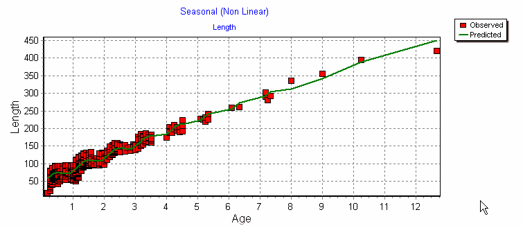
Use File|Open to find and open individual sole lengths.csv (saved by default during installation in the folder C:\Program files\GrowthII\GrowthDemoData).

From the Seasonal Age/Size drop-down select Seasonal which will fit a curve to the individual data points. Note that this fit is not very impressive because almost all the data are for the youngest ages and there is insufficient data for sole above 5 years of age to give a good fit.

Our final examples use data from Cubillos et al (2001). Because the data points were read from the published graphs and could not be accurately acquired we will not get exactly the same fit as the authors, but we can demonstrate similar results and show the quality of fit to data sets that include data close to the asymptotic length, and do not show a winter decline in size.

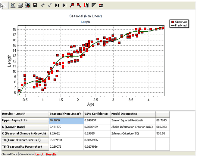
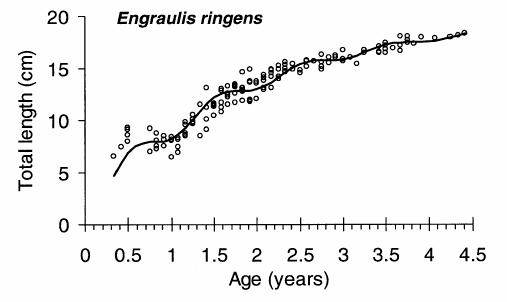
Use File|Open to find and open engraulis seasonal.csv and run a seasonal model. You will obtain the following fit:

For comparison here is the published graph

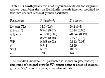
The published parameters for Engraulis ringens are shown in the table below. The authors replace TS by the Winter Point (WP) = TS+0.5 and gives the winter point at which growth is slowest. Our results indicate that WP = 0.289+0.5 = 0.789 where as the published value is 0.312. The authors argued that the slowest growth rate occurred prior to the southern hemisphere winter in April-May. Our result (using less accurate data suggests lowest growth in occurred in late winter (September 9/12 = 0.75). It is easy to see the cause of this discrepancy as for an extended period the fish grow little and during their first winter appear to shrink. Thus TS is easily changed by small alterations in the data.

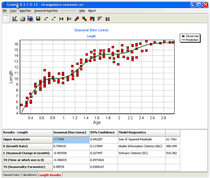
As our final example use File|Open to find and open strangomera seasonal.csv and run a seasonal model. You will obtain the following fit:

The published parameters for these data, which are similar to those calculated by Growth II, are shown in the table above.